I. INTRODUCTION
In these days, automobiles have become an essential part of everyday life. According to the 2023 National Police Agency Statistical Yearbook of South Korea, the number of registered vehicles reached 25,949,201 in 2023, more than 12 times the 2,035,448 registered in 1988 [1]. It not only reflects South Korea’s economic growth and improved living standards over the past 40 years but also serves as a crucial indicator of how deeply cars are involved in modern life.
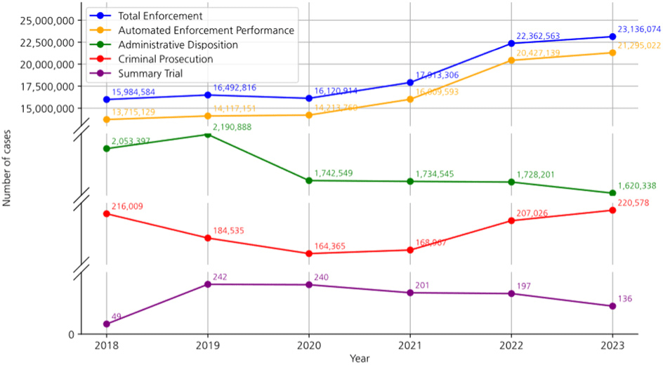
However, the increase in the number of vehicles has led to various social problems. In particular, traffic congestion and the rise in traffic accidents are causing serious concerns. The annual vehicle enforcement and processing data presented in Fig. 1 reveals that vehicle enforcement has increased in direct proportion to the number of vehicles, suggesting a sustained high risk of traffic law violations and consequent accidents.
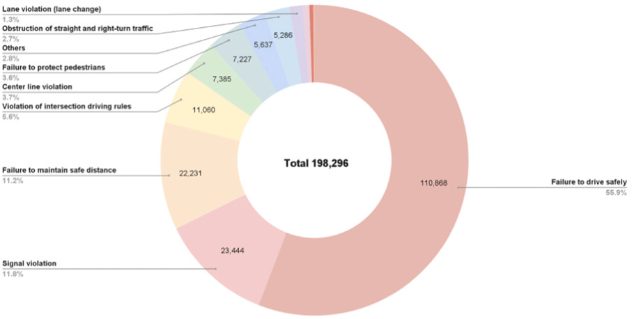
As depicted in Fig. 2, the analysis of traffic accident causes in 2023 reveals that failure to drive safely accounted for 55.9% of all accidents, followed by signal violations at 11.8% and failure to maintain a safe distance at 11.2%. These statistics clearly show that driver negligence is the main cause of most traffic accidents. Therefore, along with improving driver’s safety awareness, technological solutions are needed.
Recent advances in computing power and deep learning technology have made real-time object detection possible. This technological progress is opening up new possibilities in the field of traffic safety. In particular, traffic CCTV cameras installed throughout cities provide suitable infrastructure for applying these advanced technologies.
In South Korea, traffic law violations (e.g., speeding, signal violations) are enforced by Automatic Vehicle Identification (AVI) systems like ANPR [2]. However, current systems do not separately analyze traffic volume, and hence the ITS National Transport Information Center uses only driving speed, not volume, to determine traffic flows.
Table 1 presents the traffic map legend of the ITS National Transportation Information Center, classifying traffic flows according to speed for each road type.
| (km/h) | Urban | Rural | Urban expressway | Highway |
|---|---|---|---|---|
| Smooth | 25≤ | 50≤ | 50≤ | 80≤ |
| Congested | 15−25 | 30−50 | 30−50 | 40−80 |
| Stopped | 15> | 30> | 30> | 40> |
Modern urban traffic monitoring systems have become essential for efficient traffic management and safe road environments. However, as these systems evolve, new challenges are emerging. This research aims to address two major issues faced by current traffic monitoring systems.
The first issue concerns the balance between effective vehicle tracking and personal privacy protection [3-4]. Current Automatic Number Plate Recognition (ANPR) systems, while effective for traffic law enforcement and crime investigation, raise serious privacy concerns. These systems can potentially expose not only vehicle location information but also individual’s daily movement patterns, visited places, and lifestyle habits. Related articles suggest that such systems can track the movements of all people, not just criminals, and may violate constitutional protections against unreasonable searches [5].
The second issue relates to the limitations of existing anomaly detection methods in traffic CCTV footage. Current methods, such as Mixture of Gaussian (MoG2) [6], Optical flow [7], and Decision Trees [4], involve complex and labor-intensive preprocessing steps like lane masking [8, 9]. These approaches face several challenges, including performance degradation in complex backgrounds, increased computational costs, overfitting, and difficulties in generalizing across diverse traffic environments and conditions [10].
To address these challenges, this research sets two primary objectives. First, we aim to develop a real-time vehicle detection and tracking system that protects privacy. Inspired by vehicle re-identification research [11], we propose utilizing vehicle appearance features to track individual vehicle movements without relying on license plates. This approach seeks to achieve both personal information protection and effective vehicle detection simultaneously.
Second, we aim to identify anomalous traffic flows through similarity comparisons of vehicle trajectories. This trajectory similarity-based approach has the potential to detect anomalies in various traffic situations without complex preprocessing or environment-specific modeling. We intend to use this technology to identify abnormal traffic flows such as congestion and stopping.
By pursuing these objectives, we aim to develop a system that enables effective traffic monitoring while protecting individual privacy, and to present a generalized anomaly detection method applicable to diverse traffic environments. This research is expected to contribute significantly to advancing modern urban traffic management systems, striking a balance between efficient monitoring and privacy protection while offering a more versatile approach to anomaly detection in traffic flows.
This paper extends existing research by proposing a novel system that analyzes traffic conditions through vehicle trajectory similarity using deep learning techniques and CCTV data. The key contributions of this research are twofold. First, it emphasizes real-time traffic monitoring while considering privacy protection, addressing a critical gap in current intelligent transportation systems (ITS). This research leverages trajectory similarity to provide a more comprehensive and privacy-conscious approach to traffic flow analysis. Second, it introduces a trajectory similarity-based approach designed to detect anomalous traffic flows across diverse environments without complex preprocessing, enhancing the applicability of traffic monitoring systems.
The structure of this paper is as follows: Section II reviews related work in the field. Section III details methodology employed in this research. Section IV presents and discusses the results of experiments. Finally, Section V concludes the paper with a summary of findings and implications for future research.
II. RELATED WORKS
Deep learning-based object detection models can be broadly categorized into Convolutional Neural Networks (CNN) [12] based models, Vision Transformer (ViT) [13] based models, and Hybrid models that combine these two approaches. Recently, End-to-End models like the Detection Transformer (DETR) [14] series have also gained attention.
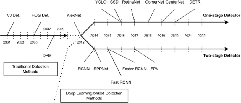
CNN-based models recognize object by extracting local and hierarchical features from input images [15]. CNNs are divided into two-stage detectors and one-stage (Single-stage) detectors [16]. Fig. 3 illustrates the roadmap of object detection from 2000 to 2022, providing a comprehensive overview of the evolution of object detection techniques over the past two decades. This timeline showcases the progression of CNN-based models and highlights the development of both two-stage and one-stage detectors, offering a clear visual representation of how object detection methods have advanced and diversified over time.
Two-stage detectors go through a region proposal stage and a classification and refinement stage. They provide high accuracy but are relatively slow in processing speed [15,17]. One-stage detectors predict the location and class of objects in a single pass through a neural network. They are faster but may have slightly lower accuracy compared to Two-stage detectors [18].
YOLO [17] divides an image into grids and detects objects in each grid cell by processing the entire image at once to predict object locations and classes [15]. It is suitable for real-time object detection due to its fast-processing speed and low computational resource usage. Although earlier versions struggled with small and dense object detection, recent versions have significantly improved [16]. However, their performances also heavily depend on training data quality and diversity.
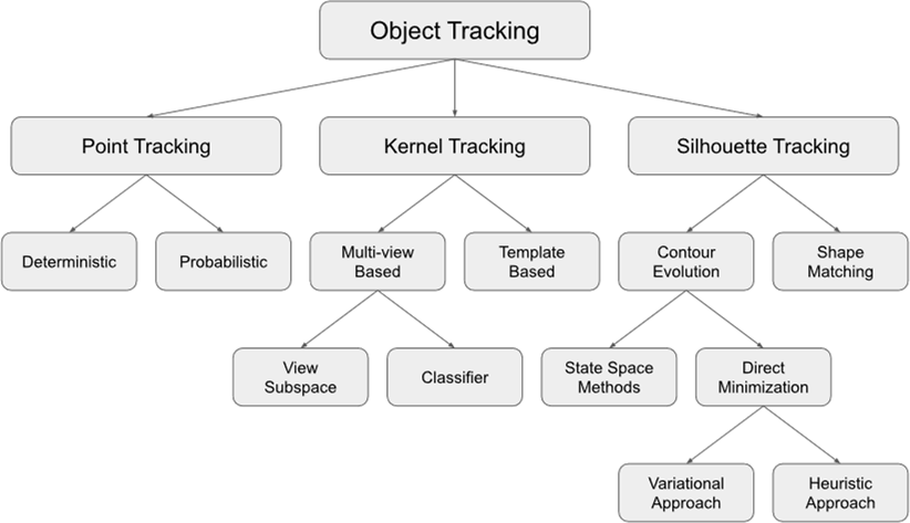
In the field of computer vision, object tracking models can be broadly categorized into point tracking, Kernel tracking, and Silhouette tracking. Fig. 4 illustrates the classification of object tracking methods.
Point tracking represents objects as one or multiple points and finds the correspondence of these point in consecutive frames. Kernel tracking represents the shape and appearance of objects as kernels like rectangles and estimates the movement of these kernels in consecutive frames. It is suitable for more complex object tracking as it can utilize object appearance information. Silhouette tracking tracks the contour or entire region of an object. It is useful for tracking non-grid objects as it can track detailed changes in object shape (Table 2).
Simple online and realtime tracking (SORT) [20], a point tracking method, uses a Kalman filter [21] to predict object position and velocity, and the Hungarian algorithm [22] to associate detected objects with predicted tracks. It uses the Intersection over union (IoU) metric to measure object association and is an online algorithm capable of real-time processing. It shows fast processing speed as it does not apply deep learning and has a simple structure. However, its performance may degrade in long-term occlusion or complex scenes as it does not consider appearance features [20].
ByteTrack [23] improves tracking performance by applying BYTE logic to SORT. It first associates detection results with confidence scores above a threshold to existing tracks, and then performs additional association using results with lower confidence scores. Due to the BYTE logic, it is fast and efficient, enabling real-time processing. It can also maintain object continuity well in complex scenes.
Latest innovations in intelligent transportation systems (ITS) have emphasized the development of real-time traffic flow analysis frameworks combining multi-target tracking algorithms with deep learning.
A study on real-time traffic flow analysis [24] proposed a framework combining multi-target tracking algorithms with an improved long short-term memory (LSTM) [25] network to estimate vehicle counts, speed and density. The system utilized YOLOv5 [26] for vehicle detection and DeepSORT [27] for tracking, integrating spatial-temporal features to enhance counting accuracy. By avoiding complex multi-target associations, the method achieved an average processing speed of 45.22 FPS while maintaining 96.58% accuracy in bidirectional vehicle counting under diverse scenarios. However, performance degradation was observed in low-visibility conditions, underscoring difficulties in environmental adaptability.
A study on real-time vehicle tracking [28] addressed challenges in complex traffic environments by integrating YOLOv5 with DeepSORT. This approach reduced ID switches by leveraging motion and appearance descriptors, achieving 95.3% precision in vehicle tracking at 32 FPS. To enhance robustness, Kalman filtering and the Hungarian algorithm were employed for state estimation and data association. While the system demonstrated high performance in crowded scenes, limitations included reduced accuracy for small-scale vehicles and dependency on high-quality detection inputs.
A study on optimizing traffic management system [29] introduced YOLOv8 [30] as an upgraded detector paired with DeepSORT to improve vehicle tracking stability. The framework utilized feature pyramids in YOLOv8 for multi-scale detection and incorporated spatial attention mechanisms to reduce missed detections. Evaluated on the MS COCO dataset [31], the model achieved a 0.78 mAP@0.5 and reduced ID switches by 18% compared to earlier YOLO versions. In spite of its real-time efficiency, the system grappled with occluded vehicles in adverse weather and needed further training on diverse datasets for broader applicability.
A study on intelligent surveillance systems [32] explored the use of CNNs and RNNs for real-time anomaly detection in traffic videos. The framework combined object detection using Faster R-CNN [33] with temporal analysis via LSTM networks to identify abnormal behaviors, achieving 97.6% accuracy in accident detection. This system emphasized edge-based processing to reduce latency, enabling deployment on low-cost hardware. Key limitations contained high computational demands for high-resolution videos and privacy concerns connected to continuous monitoring.
III. METHODOLOGY
Fig. 5 illustrates the proposed similarity-based real-time traffic flow analysis pipeline. This pipeline is designed to analyze traffic conditions in real-time using CCTV footage and consists of key stages, including object detection, vehicle tracking, trajectory similarity computation, grouping and visualization.
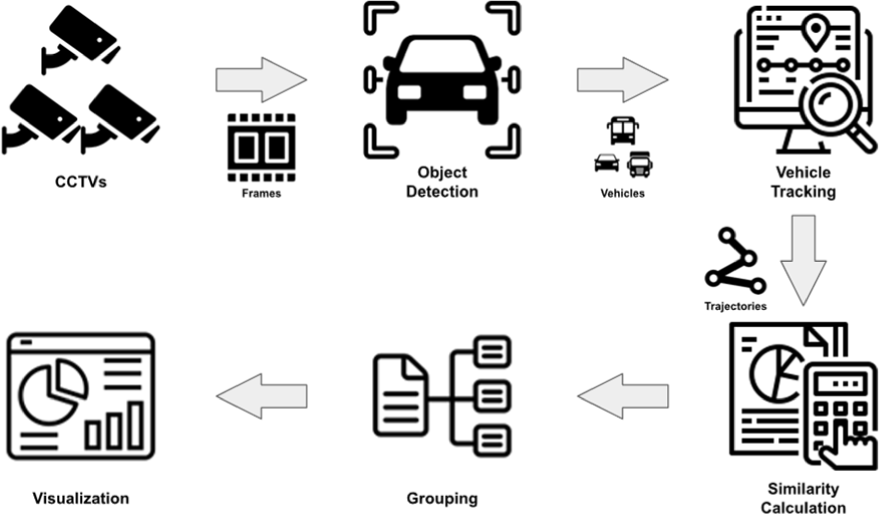
First, objects are detected from CCTV footage using a YOLO model which is a one-stage detector and well-suited for real-time object detection due to its speed and efficiency. If the detected objects belong to vehicle classes (car, bus, and truck), tracking begins using the ByteTrack algorithm. It performs tracking in two-stages based on confidence scores. In the first stage, objects with confidence scores above a threshold are classified into the ‘High Confidence’ group and track initially. In the second stage, objects with confidence scores below the threshold are classified into ‘Low Confidence’ group and undergo additional tracking. This dual-stage tracking mechanism ensures stable tracking performance even in highly congested situations.
The trajectory data of tracked vehicles consists of frame ID, object ID, and the x and y coordinates of the bounding box’s center point. The center point of the bounding box is used because it represents a geometric average, providing more stable results during trajectory generation. The generated trajectory data undergoes preprocessing before computing trajectory similarity between object IDs. The similarity metrics used include Cosine Similarity, Jensen-Shannon Divergence, and Euclidean Distance. If all three similarity values exceed their respective thresholds, the corresponding object IDs are grouped together. Finally, trajectories belonging to the same group are visualized in the same color to facilitate traffic flow analysis.
The following subsection provides detailed explanations of each stage and research methodology.
In this study, 17,003 validation images from the ‘CCTV Traffic Video (Highway) for Solving Traffic Problems’ [34] provided by AI-Hub were utilized for evaluating the performance of YOLO models to select the most suitable real-time object detection model for traffic flow analysis. This dataset features high-quality FHD resolution and consists of a total of 505 hours of video footage and 500,000 images. Specifically, it provides 300,000 bounding box images and 200,000 segmentation images.
This dataset classifies vehicles into three categories as car, truck and bus. The data was collected from 50 different CCTV locations, covering diverse road environments such as general roads for 60%, bridges for 35%, and tunnels for 5%. Time periods are distributed as follows: daytime accounts for approximately 68%, nighttime for 22%, and dawn for 9%. Weather conditions include clear skies for 83%, rain for 11%, fog for 4% and snow for 3%.
The dataset provides labels in XML format, which required preprocessing to make them compatible with YOLO models. Using python scripts, the XML labels were converted into YOLO format by generating txt files for each image such as the Class ID, x and y coordinates, width, and height of each bounding box. This preprocessing ensured that high quality traffic CCTV data could be effectively utilized for YOLO model performance evaluation.
The diversity in road types, time periods, and weather conditions makes this dataset highly suitable for training and evaluating object detection models in realistic traffic environments. By leveraging this dataset, the study aimed to identify the most effective YOLO model for real-time traffic flow analysis.
The YOLO models evaluated in this study include YOLOv5 [26], YOLOv6 [35-36], YOLOv7 [37], YOLOv8 [30], YOLOv9 [38] and YOLOv10 [39].
The evaluation metrics used in this study are mAP@0.5 (mean Average Precision at IoU 0.5) and FPS (Frames Per Second), which measure the accuracy of object detection and real-time processing capability, respectively. The mAP@0.5 represents the mean Average Precision when the intersection over union (IoU) threshold is set to 0.5. It is a standard metric for evaluating the accuracy of object detection models and is calculated as following formula (1):
where, n is the number of classes, and APi denotes the Average Precision for each class.
The FPS measures the number of frames a model can process per second, reflecting its real-time performance. It is calculated as following formula (2):
In this study, both mAP@0.5 and FPS were comprehensively considered to select the optimal model. Specifically, rankings were assigned to each model based on their mAP@0.5 and FPS values, and the average of these rankings was calculated to determine the best performing model. By adopting this approach, the study ensures that the selected model balances high detection accuracy with real-time processing capability, meeting the requirements of contemporary traffic monitoring systems.
Table 3 summarizes the hyperparameter settings used for evaluating YOLO models for each metrics. ‘Batch Size’ defines the number of images processed in a single inference batch. For FPS measurements, the batch size was set to 1 to simulate real-time streaming environments where frames are processed one at a time. ‘Image Size’ refers to the resolution of input image fed into the model. YOLO models generally require an input resolution of 640×640 pixels for optimal performance. ‘Confidence Threshold’ sets the minimum confidence score required for a detection to be considered valid. Only detections with confidence scores above this threshold are treated as true objects. ‘IoU Threshold’ specifies the intersection over Union threshold used to evaluate detection accuracy by measuring the overlap between predicted bounding boxes and ground truth objects. ‘Half Precision’ determines whether half-precision floating-point calculations are used during inference. Enabling this parameter reduces memory usage and increases computational speed but may slightly impact accuracy. ‘Number of Images’ indicates the total number of images used for evaluating each model’s performance.
| mAP@0.5 | FPS | ||
|---|---|---|---|
| Batch size | 32 | 1 | |
| Image size | 640 | ||
| Confidence threshold | 0.001 | 0.25 | |
| IoU threshold | 0.6 | 0.45 | |
| Half precision | False | ||
| Number of images | 17003 |
In this study, the tracking images from the ‘CCTV Traffic Video (Urban Roads) for Solving Traffic Problems’ [40] provided by AI-Hub were utilized for traffic situation analysis. This dataset features high-quality FHD resolution and includes a total of 505 hours of video footage and 570,000 images. Specifically, it provides 180,000 bounding box images, 30,000 segmentation images, and 360,000 tracking images.
The tracking data contains information that can be effectively utilized for traffic analysis. Each frame includes bounding box coordinates for object locations along with an object ID to uniquely identify each object. Additionally, the category ID specifies the object class. The data is structured in JSON format and includes metadata such as the image file name, capture time, and frame ID, enabling efficient data management and analysis.
Notably, this dataset reflects real-word traffic environments by including various time periods (daytime and nighttime) and weather conditions (clear skies, rain, etc.). These characteristics make it highly suitable for model training and evaluation. It also applicable to a wide range of research purposes such as traffic flow analysis, vehicle tracking, and anomaly detection.
The vehicle tracking performance in this study was evaluated using a model that combines the best performing object detection model from the YOLO model evaluation and ByteTrack for tracking.
The hyperparameter configurations used in the vehicle detection and tracking model are the default values set in the model, and these values are summarized in Table 4. While optimizing these hyperparameters could potentially yield best performance, we choose to use the default values to ensure a fair comparison across various models. This approach allows for an unbiased evaluation of each model’s baseline performance without the advantage of model-specific tuning. The ‘Confidence Threshold’ and ‘IoU Threshold’ follow the same settings as described in Table 3, which were used for FPS measurement. ‘Track Threshold’ determines whether an object’s confidence score qualifies it to be classified into the ‘High Confidence’ group in ByteTrack’s BYTE logic. Objects with scores below this threshold are considered ‘Low Confidence’ group and are handled differently during tracking. ‘Match Threshold’ sets the similarity threshold required to match detections in the current frame with tracks from previous frames. Only matches exceeding this threshold are considered valid, ensuring accurate association between frames. ‘Aspect Ratio Threshold’ limits the allowable aspect ratio of detected objects. Bounding boxes with aspect ratio exceeding this threshold are excluded from tracking, preventing anomalies cause be irregularly shaped detections. ‘Min Box Area’ specifies the minimum pixel area for bounding boxes. Detections smaller than this value are ignored to reduce noise and improve tracking reliability.
| Confidence threshold | 0.25 |
|---|---|
| IoU threshold | 0.45 |
| Track threshold | 0.5 |
| Match threshold | 0.7 |
| Aspect ratio threshold | 3.0 |
| Min box area | 36 |
The evaluation metrics used to assess tracking performance are MOTA (multiple object tracking accuracy) [41, 42], MOTP (multi-object tracking precision) [41], and IDF1 (Identity F1 Score) [42]. MOTA evaluates overall tracking performance by considering both detection accuracy and ID assignment consistency across frames [41]. It is calculated as following formula (3):
where FN represents the number of missed objects, FP denotes the number of false detections, IDSW indicates the number of ID switches, and GT refers to the total number of ground truth objects. A higher MOTA value, closer to 1, indicates better tracking performance. However, MOTA does not consider the accuracy of object locations and only penalized ID switches once per occurrence, which may lead to an overestimation of performance in complex scenarios [41].
MOTP measures how accurately tracked object positions align with ground truth locations. It is calculated as following formula (4):
where represents the sum of IoUs for all matched object pairs and ct denotes number of matches at time t. For IoU-based MOTP, values closer to 1 indicate higher precision. MOTP focuses on spatial precision but does not consider ID consistency.
IDF1 evaluates how consistently IDs are maintained across frames by balancing precision and recall of ID assignments. It is calculated as following formula (5):
where IDTP represents correctly identified objects, IDFP denotes incorrectly identified objects, and IDFN indicates missed objects. Unlike MOTA and MOTP, IDF1 considers long-term ID consistency, making it particularly useful for evaluating complex tracking scenarios. However, it may oversimplify some cases by relying on fixed IoU thresholds [42].
To calculate the evaluation metrics, IoU-based distance measurements were used to match ground truth labels with the model’s predictions. In cases where different IDs were assigned to the same object, the bounding box information for each frame was stored in a dictionary using the object ID as the key. Subsequently, the Hungarian algorithm [22] was applied to find the optimal matching between ground truth trajectories and predicted trajectories.
We generate vehicle trajectories every 60 seconds. To calculate trajectory similarity, the metrics used in this study include Cosine Similarity [43], Jensen-Shannon Divergence [44] and Euclidean Distance Similarity [45]. Each metric evaluates different aspect of trajectory similarity. ‘Cosine Similarity’ compares the similarity in movement direction, ‘Jensen-Shannon Divergence’ assesses the similarity in movement patterns, and ‘Euclidean Distance Similarity’ measures the positional similarity between trajectories. Since these metrics require data of equal length, shorter trajectories are padded with zeros to match the length of the longer trajectories.
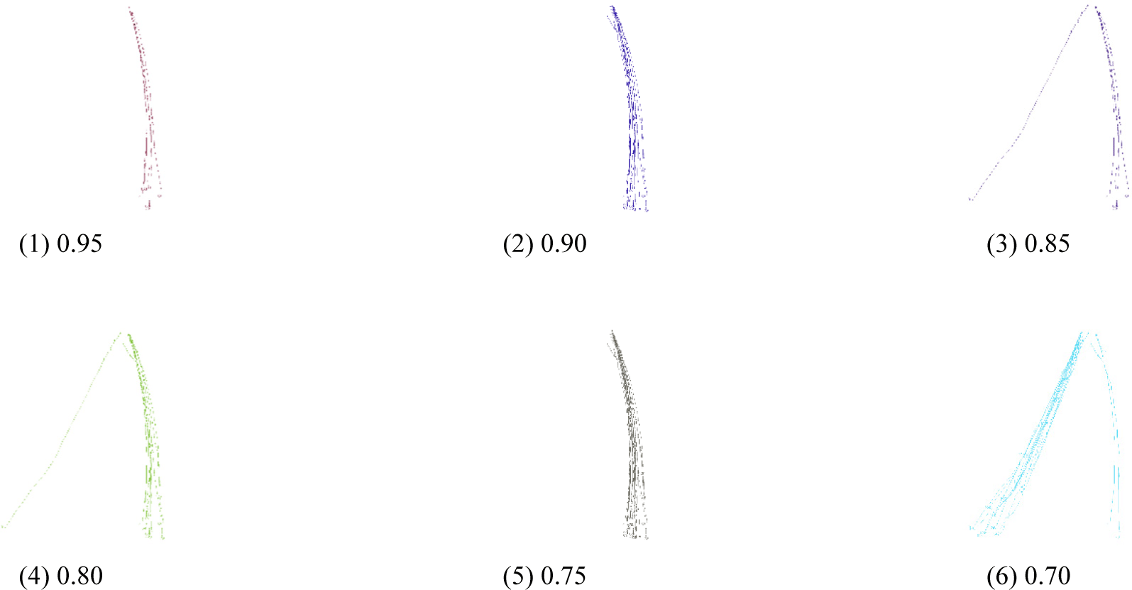
Table 5 summarizes the hyperparameter settings used for trajectory similarity-based grouping in traffic flow analysis. ‘Similarity Threshold’ determine whether objects are grouped into the same group based on their similarity scores. The thresholds were tested at intervals from 0.70 to 0.95 in steps of 0.05 for comprehensive performance evaluation. For Euclidean Distance Similarity, the threshold values were divided by 100 to normalize them due to their larger value ranges compared to other metrics.
| 1 | 2 | 3 | 4 | 5 | 6 | |
|---|---|---|---|---|---|---|
| Similarity threshold | 0.95 | 0.90 | 0.85 | 0.80 | 0.75 | 0.70 |
These hyperparameter values were determined through preliminary experiments and may need adjustment based on specific road characteristics such as vehicle speed, road length, road shape, and traffic volume during real-world applications.
All similarity values are normalized to a range between 0 and 1, where values closer to 1 indicate higher similarity between trajectories. If all three metrics exceed their respective threshold, the two trajectories are grouped into the same group. This method ensures that only highly similar trajectories are grouped together, providing robust basis for traffic flow analysis.
Cosine Similarity is used in various fields such as document clustering and search engine optimization, and is particularly effective in analyzing text data in high-dimensional spaces [43]. It measures the similarity of angles between two vectors, ignoring the magnitude of the vectors and considering only the direction. This allows reflecting the relative importance of words rather than the absolute difference in document length or word frequency. Cosine Similarity is calculated as following formula (6):
where A and B are vectors to be compared. Cosine Similarity has a time complexity of O(n), where n is the number of dimensions of the vector. Cosine Similarity takes values between −1 and 1, where 1 indicates the same direction, 0 indicates orthogonality, and −1 indicates opposite directions. In this study, to normalize it to a range 0 and 1 for consistent comparison, a linear transformation is applied.
Jensen-Shannon Divergence (JSD) is widely used in information theory and machine learning [44]. It measures the similarity between two probability distributions base on Kullback-Leibler Divergence [46], but it has the advantages of being symmetric and always yielding a finite value. These characteristics make it easier to interpret than Kullback-Leibler Divergence, especially when differences between distributions are small or when noise is present. It is calculated as following formula (7):
where KL represents the Kullback-Leibler Divergence, JSD denotes the Jensen-Shannon Divergence, P and Q are the two probabilities distribute being compared. M is equal to the sum of P and Q divided by 2. Jensen-Shannon Divergence has a time complexity of O(n), where n is the number of elements in the probability distribution. JSD ranges from 0 to ln (2), with values closer to 0 indicating higher similarity between distributions. In this study, to normalize it to a range between 0 and 1 for consistent comparison, reciprocal and complement transformations were applied.
Euclidean Distance Similarity is mainly used in pattern recognition, image processing, and cluster analysis [46]. Euclidean Distance Similarity measures the similarity of the straight-line distance between two vectors and is calculated as follows:
where EDS represents Euclidean Distance Similarity, P and Q are two points in n-dimensional space, and D(P,Q) represents the Euclidean Distance between these two points. Due to its sensitivity to magnitudes, Euclidean Distance Similarity (ranging from 0 to 1, with 1 being highest similarity) requires proper data scaling. Its time complexity is O(n), where n is the vector’s dimensionality.
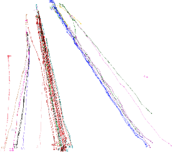
The trajectories of objects were visualized by connecting the center coordinates of their bounding boxes in each frame. To illustrate changes in vehicle speed, points were marked at 1 second intervals. Each object ID was displayed next to the final coordinate to indicate the direction of the vehicle’s movement. Objects belonging to the same group were distinguished using the same color, providing clear visual differentiation.
Fig. 6 shows the trajectories of vehicles collected from a dataset. Wider gaps between points indicate higher vehicle speeds, while narrower gaps represent slower speeds. This visualization method allows for an intuitive understanding of the movement paths of vehicles over time and the relationship between different groups.
The experimental environment used in this study is detailed in Table 6. It consists of a high-performance system equipped with AMD Ryzen 7 7700 CPU, NVIDIA GeForce RTX 4070 Ti GPU, and 32 GB of DDR5 5,600 MHz RAM. This system runs on the Windows 11 operating system and utilizes Python 3.8.10 and PyTorch 2.2.1 to handle large-scale and complex computations. Additionally, CUDA 12.1 is supported to optimize GPU acceleration for enhanced performance.
| HW | CPU | AMD Ryzen 7 7700 8 Core 3.80 GHz |
| GPU | NVIDIA GeForce RTX 4070 Ti | |
| RAM | DDR5 5,600 MHz 32 GB | |
| SW | OS | Windows 11 |
| Python | 3.8.10 | |
| CUDA | 12.1 | |
| Pytorch | 2.21 |
IV. RESULTS
Table 7 presents the results of evaluating the performance of YOLO models. Among the evaluated models, YOLOv7x, YOLOv7, YOLOv5x, YOLOv5l, YOLOv9c, YOLOv5m, YOLOv7-tiny, YOLOv5s and YOLOv5n demonstrated FPS values exceeding 60, making them suitable for real-time object detection. Notably, YOLOv7x demonstrated the best performance with a mAP@0.5 of 0.708 and FPS of 87.9843.
The vehicle tracking performance was evaluated using a model that combines YOLOv7x for object detection and ByteTrack for tracking. Table 8 presents the results of the vehicle tracking performance evaluation.
| Metric | Value |
|---|---|
| MOTA | 0.289158 |
| MOTP (IoU) | 0.836673 |
| IDF1 | 0.725077 |
The evaluation results indicate that the YOLOv7x and ByteTrack combination achieves a MOTA of 0.289158, reflecting moderate overall tracking accuracy by considering missed detections, false positives, and ID switches. The MOTP score of 0.836673 demonstrates high spatial precision in aligning tracked objects with their ground truth locations. Additionally, the IDF1 of 0.725077 highlights strong consistency in maintaining object identities across frames.
The tracking results are saved as a text file, as shown in Table 9. Each row contains information about the frame ID, object ID, and the x and y coordinates of the bounding box’s center. This data serves as the basis for generating other metrics, the high MOTP and IDF1 values suggest that the model excels in precise object localization and Identity preservation, which are critical for effective vehicle tracking in dynamic traffic environments.
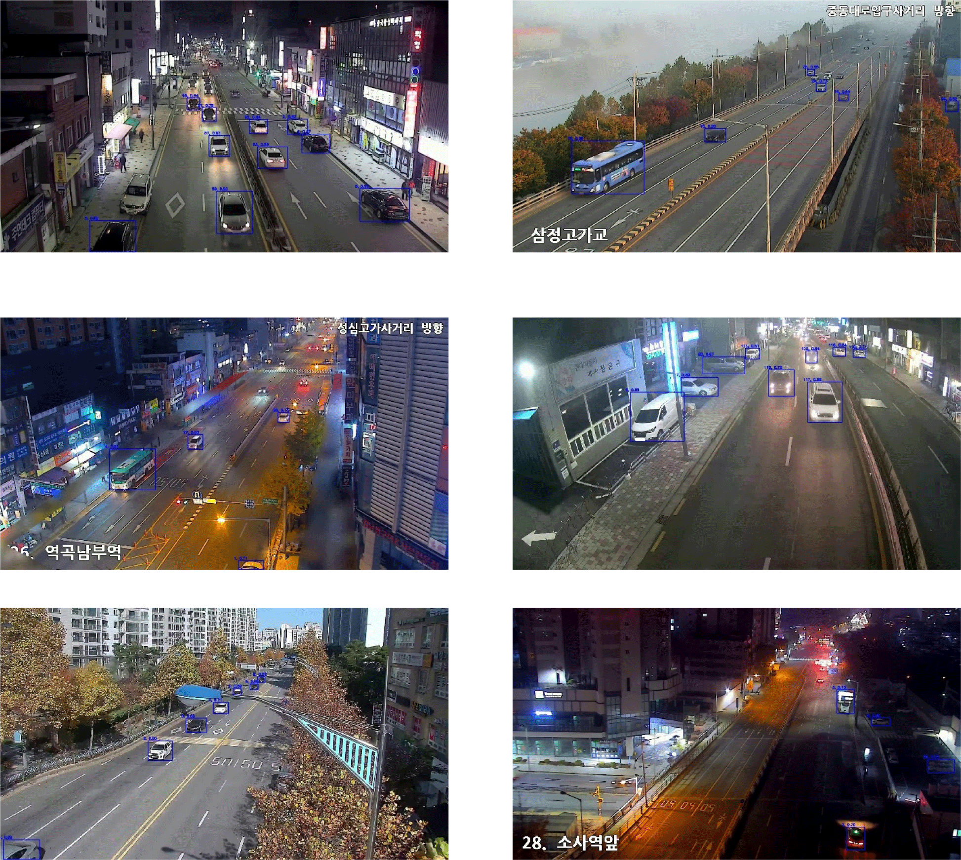
Fig. 7 shows the results of vehicle tracking performed using YOLOv7x and ByteTrack. The CCTV footage visualizes bounding boxes, object IDs, and confidence scores for each detected vehicle. The bounding boxes represent the detected vehicle’s position, while the object IDs indicate unique identifiers assigned to each tracked vehicle to ensure continuity across frames. The confidence scores, displayed next to the object IDs, reflect the model’s certainty in detecting the corresponding objects.
The visualization highlights the effectiveness of YOLOv7x and ByteTrack in accurately detecting and tracking vehicles under various conditions, including daytime and nighttime scenarios.
The tracking results are saved as a text file, as shown in Table 9. Each row contains information about the frame ID, object ID, and the x and y coordinates of the bounding box’s center. This data serves as the basis for generating vehicle trajectories.
Using this tracking data, trajectory similarity was calculated based on three metrics. The results are presented in Table 10. In this table, ID 1 and ID 2 represent the IDs of two vehicles being compared.
Fig. 8 illustrates the results of vehicle trajectory grouping based on similarity thresholds. At lower threshold, most trajectories tended to be grouped into a single large group, indicating less differentiation between movement patterns. In contrast, higher threshold allowed for more precise grouping, effectively distinguishing vehicles with similar movement patterns.
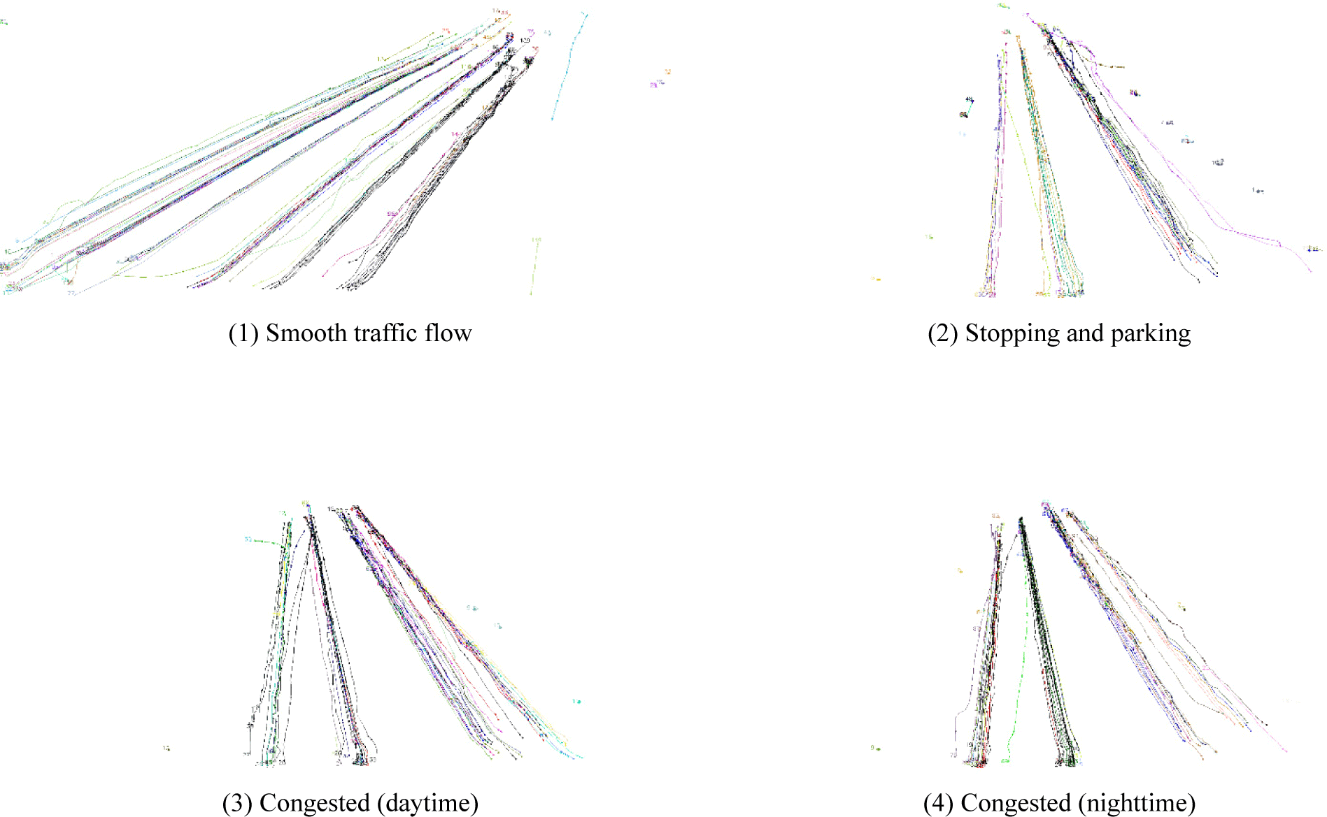
Fig. 9 illustrates the results of traffic flow analysis at a similarity threshold of 0.95. Through the visualization of vehicle trajectories, different traffic conditions were identified.
In smooth traffic flow situation, vehicle trajectories maintained relatively consistent spacing and continuity, indicating smooth and uninterrupted movement. In stopping and parking Situations, vehicle trajectories appeared as isolated points, making it easy to distinguish stationary vehicles. In congested traffic situation, vehicle trajectories were shorter, with narrower and irregular spacing compared to smooth traffic conditions, reflecting slower vehicle movements.
While the current analysis provides valuable qualitative insights into vehicle trajectories and traffic flows, it lacks quantitative performance metrics for trajectory grouping and traffic flow analysis. To address this limitation and enhance the robustness of our results, we propose introducing new metrics in future research.
We plan to develop a comprehensive metric called “Trajectory Precision” that combines multiple object tracking precision (MOTP) with a new measure we term “Group Precision”. This metric will provide a quantitative assessment of both tracking accuracy and the effectiveness of trajectory grouping.
To implement this new metric, we will need to expand our dataset by adding “group ID” labels to the tracking data. This additional labeling will allow us to evaluate how well our grouping algorithm aligns with ground truth group assignments. However, further discussion is needed on how to effectively label these “group ID” s, as this process may require careful consideration and potentially new methodologies.
The introduction of these quantitative metrics will signif-icantly enhance our ability to evaluate and compare different trajectory grouping methods and provide a more objective assessment of traffic flow analysis.
V. CONCLUSION
This study proposed a traffic flow analysis method based on deep learning by comparing vehicle trajectory similarities. Through the evaluation of YOLO model performance, the most suitable model for real-time vehicle detection was selected. As a result, the YOLOv7x model demonstrated superior performance, achieving mAP@0.5 of 0.708 and FPS of 87.9843, confirming its suitability as a real-time vehicle detection model.
Using YOLOv7x as the object detection model and ByteTrack as the object tracking model, vehicle detection and tracking were performed, followed by an evaluation of tracking performance. This combination achieved a MOTA of 0.289158, a MOTP of 0.836673, and an IDF1 of 0.725077. These results demonstrate stable tracking performance under specific conditions, highlighting its potential for application in real-time traffic analysis.
Vehicle trajectories were generated through vehicle detection and tracking, and trajectory similarities were analyzed using Cosine Similarity, Jensen-Shannon Divergence, and Euclidean Distance metrics. By combining these three-similarity metrics, comprehensive evaluations of vehicle movement direction, patterns, and positional similarities were achieved. Additionally, grouping results based on similarity thresholds were visualized to provide an intuitive method for understanding various traffic situations.
The proposed method minimizes privacy concerns while enabling effective traffic flow analysis and supports real-time processing. However, this study has limitations as experiments were conducted only in limited road environments, and performance under extreme conditions such as severe weather was not verified. Furthermore, the method does not include to detect vehicles exhibiting abnormal behaviors such as sudden lane changes or stopping due to accidents.
In future research, we aim to address the current limitations by expanding the dataset and improving model performance through cutting-edge methodologies. A key challenge lies in acquiring data for extreme weather conditions and accident scenarios, which are scarce in real-world settings. To tackle this, we propose leveraging Generative Adversarial Networks (GANs) to create synthetic imagery. These artificially generated images will serve as supplementary training data, bolstering the model’s capacity to navigate a broader spectrum of real-life traffic situations. Additionally, we plan to integrate deep learning-based anomaly detection algorithms to pinpoint atypical vehicle trajectories. The synergy between GAN-synthesized data and anomaly detection techniques is expected to improve the model’s accuracy in managing infrequent yet pivotal events, such as abrupt lane shifts or collisions. These technological introductions are expected to play a crucial role in advancing the development of next-generation smart cities and intelligent transportation system (ITS).


