I. INTRODUCTION
In South Korea, the number of patients with brain tumors has increased by approximately 30% over four years, from approximately 49,000 in 2017 to approximately 64,000 in 2021 [1]. Typically, the diagnosis of brain tumors involves the manual delineation of tumor areas by specialists based on brain images obtained using magnetic resonance imaging (MRI) [2]. However, this method is time-consuming and may be influenced by the diagnostician’s skills and errors. Computer-aided diagnostic methods have garnered considerable attention for addressing these challenges. Among these, the application of deep-learning-based image segmentation has been actively researched owing to its accuracy and simplicity [3].
U-Net is a prominent CNN-based deep learning model widely employed in medical image segmentation, achieving high accuracy through its encoder-decoder architecture and utilization of skip connection techniques [4]. U-Net has been consistently researched in the field of brain tumor image segmentation, with numerous models in this domain based on the U-Net structure.
The U-Net architecture is categorized into two-dimensional (2D) and three-dimensional (3D) U-Net based on dimensionality, each possessing distinct advantages. The 2D U-Net incurs lower computational costs owing to the smaller number of parameters used in the model. On the other hand, 3D U-Net, unlike the 2D structure, can utilize inter-slice information, enabling more accurate segmentation [5].
However, in medical image segmentation using U-Net models, there is often no significant difference between 2D and 3D U-Net, or 2D U-Net sometimes performs better [6-9]. We hypothesize that this is due to the decreased performance of batch normalization with small batch sizes.
Batch Normalization included in the basic structure of U-Net contributes to model performance improvements [10], but it may not perform well when the batch size is too small [11]. The high computational cost of 3D U-Net, which makes it challenging to set a large batch size, therefore, might lead to a decrease in performance. In such cases, replacing batch normalization with alternative normalization methods that are not affected by batch size, such as group normalization or instance normalization, could be a solution [11-12].
However, we found that most studies comparing 2D U-Net and 3D U-Net applied batch normalization to the 3D models.
Therefore, this study conducted a comparative analysis of the brain tumor image segmentation performance between 2D U-Net and 3D U-Net employing various normalization techniques (batch normalization, group normalization, and instance normalization). Through this experiment, we aim to determine the effectiveness of replacing batch normalization with other normalization methods (group normalization and instance normalization) in 3D U-Net, and to evaluate which model, 2D U-Net or 3D U-Net, is more effective for brain tumor segmentation.
II. RELATED WORKS
Vimala et al. used the EfficientNet family (EfficientNet B0 to B4) pre-trained on the ImageNet dataset as the backbone for brain tumor detection and classification. They added simple customized layers to EfficientNet to enable tumor classification and applied transfer learning using the CE-MRI Figshare brain tumor dataset. EfficientNet B2 achieved the highest performance with an accuracy of 99.06% (98.57% before data augmentation) on tests. In cross-dataset validation using an external brain tumor classification dataset from the Kaggle repository, EfficientNet B2 also achieved the highest accuracy of 92.23% [13].
Ahamed et al. emphasized the importance of federated learning. High-performance AI tumor diagnosis requires large datasets from various sources. However, collecting medical data is challenging due to privacy concerns. Federated learning addresses this by allowing models to learn from diverse data without direct data transmission, thereby maintaining privacy while enhancing model effectiveness and generalization [14].
Almutairi et al. proposed the GTO-DQL model for breast cancer classification, achieving accuracy rates of 98.90% on the WBCD dataset, 99.02% on the WDBC dataset, and 98.88% on the WPBC dataset, outperforming traditional models such as RBF-ELB, PSO-MLP, and GA-MLP. This model utilizes Gorilla Troops Optimization (GTO) for feature extraction from the datasets and employs Deep Q Learning with a Deep Neural Network (DNN) to update Q-values for tumor classification. Finally, the Local Interpretable Model-agnostic Explanations (LIME) model is used to explain the results to the user [15].
In summary, these examples demonstrate that fine-tuning pretrained models, utilizing data augmentation techniques, and applying federated learning are effective strategies for enhancing AI models. Additionally, it is evident that reinforcement learning can be a beneficial approach in certain situations.
In 2017, Dong et al. utilized a U-Net-based FCN (fully convolutional network) model to segment the BRATS 2015 dataset. They achieved Dice scores of 0.86 for the whole tumor, 0.86 for the tumor core, and 0.65 for the enhancing tumor [16].
In 2019, Jiang et al. introduced a Two-stage Cascaded U-Net model. This architecture combines two U-Net structures, where the first U-Net segments the input data and the result is concatenated with the input data before being fed into the second U-Net for the final segmentation. The model achieved first place in the segmentation task category of the BRATS 2019 challenge, recording Dice scores of 0.89 for the entire tumor, 0.84 for the tumor core, and 0.83 for the enhancing tumor [17].
In 2020, Lee et al. [18] devised a patchwise U-Net model for brain imaging by dividing brain images into multiple patches, segmenting each patch individually, and then combining them. Although this model requires more training time owing to the need to train for a number of patches, it presents advantages such as reduced memory usage. The model demonstrated performance improvements of 3% and 10% compared with the conventional U-Net and SegNet-based approaches, respectively, recording an average Dice score of 0.93.
In the BRATS 2020 challenge, the nnU-Net, which stands for “no new U-Net,” achieved the top ranking in the image segmentation category, displaying Dice scores of 0.89 for the whole tumor, 0.85 for the core tumor, and 0.82 for the enhancing tumor [19]. nnU-Net is essentially identical to the traditional U-Net, except for the use of Leaky ReLU as the activation function instead of ReLU, and the adoption of instance normalization instead of batch normalization.
In 2022, Maji et al. introduced the AG Res-U-Net with Guided Decoder model, which exhibited superior performance compared to the Two-stage Cascaded U-Net model. This model adopts a structure applying the Guided Decoder technique to the Attention Res U-Net algorithm, incorporating the output not only from the last layer but also from internal layers of the U-Net’s decoder into the loss function for training. Utilizing the BRATS-2019 dataset for image segmentation, the model achieved Dice scores of 0.92 for the whole tumor, 0.85 for the tumor core, and 0.83 for the enhancing tumor [20].
Qin et al. proposed an improved U-Net3+ model. This model incorporates a stage residual structure into the encoder of the U-Net3+ architecture to minimize the vanishing gradient problem caused by the extensive use of ReLU layers and enhance feature extraction performance. Additionally, it replaces batch normalization and the ReLU activation function with filter response normalization and the TLU activation function, respectively, eliminating dependency on batch size and increasing learning capability. Although the performance slightly lags behind the 3D V-Net, it demonstrates excellent performance considering the significantly lower number of parameters [21].
Normalization layers smooths the loss function, enhancing the stability of model training and preventing the model from getting stuck in local optima [10].
Batch normalization normalizes the mean and variance of each mini-batch using trainable parameters γ (gamma) and β (beta), respectively [10].
Group normalization divides the channel dimension into multiple groups and normalizes the mean and variance within each group using trainable parameters γ (gamma) and β (beta) [11].
Instance normalization normalizes the mean and variance independently for each channel of each sample using trainable parameters γ (gamma) and β (beta). Instance normalization is equivalent to group normalization with a group size of 1 [22].
In the case of batch normalization, if the batch size is small, a few samples can have a significant impact on the overall statistics, causing the calculated mean and variance to not accurately reflect the true data distribution [11]. As a result, the model may fail to converge to the global optimum, potentially reducing the accuracy of the segmentation.
However, group normalization and instance normalization are not affected by batch size, allowing them to function reliably even with small batch sizes. According to He’s experiments, batch normalization performed better when the batch size was 16 or more, but group normalization outperformed batch normalization when the batch size was 8 or less [11]. In Kolarik’s study, batch normalization, group normalization, and instance normalization were compared when the batch size was 1. The results showed that group normalization and instance normalization outperformed batch normalization [12].
3D U-Net has greater potential than 2D U-Net because it can utilize inter-slice information, which is lost in the 2D approach [5]. However, in studies comparing 3D U-Net and 2D U-Net, instances where 2D U-Net performed better were found, all of which involved 3D U-Net using batch normalization despite having a small batch size or presumably small batch size.
In Nemoto’s study, both 2D U-Net and 3D U-Net achieved the same dice similarity coefficient (DSC) score of 0.990 in the segmentation of lung CT images [6]. In Srikrishna’s study, 2D U-Net showed significantly higher DSC in brain segmentation [7]. In Nemoto’s and Srikrishna’s studies, 3D U-Net used batch normalization, and while the batch size was not specified, it is presumed to be low given the equipment and patch size used in the experiments (32×128×128 in both experiments).
In Zettler’s study, segmentation of five abdominal organs showed that while 3D U-Net performed better for the pancreas, 2D U-Net had higher DSC scores for the other four organs. The batch size in this study was set to 8, and batch normalization was used [9].
In Yoo’s study, the performance of 2D and 3D U-Net was compared for the segmentation of the maxillary sinus. The DSC for 2D and 3D U-Net was 0.938 and 0.891, respectively, indicating that 2D U-Net had higher performance. The 3D U-Net used in this study employed batch normalization, with a batch size of 1 [8].
On the other hand, there were cases where 3D U-Net performed better, which occurred when batch normalization was used in 3D U-Net, but also when no normalization layer was used at all, or when other normalization layers were used instead of batch normalization.
In the 2016 study by Çiçek et al., the proposed 3D U-Net model outperformed the 2D U-Net with a DSC of 0.863 in semi-automated segmentation, compared to 0.796 for the 2D U-Net [23]. In this experiment, even though the batch size of the 3D U-Net was 1 and batch normalization was used, the 3D U-Net without any normalization layer still achieved a DSC of 0.843, showing better performance than the 2D model.
In Chen’s 2023 study, the SYNAPSE MULTI-ORGAN CT DATASET was segmented using various CNN models for comparison. It was confirmed that the 3D nnU-Net and 3D TransU-Net showed higher performance than their 2D versions (the 3D versions of nnU-Net and TransU-Net achieved DSCs of 87.33 and 88.11, respectively, while the 2D versions achieved DSCs of 82.92 and 84.36, respecttively). The batch size in this experiment was 2, and both models used instance normalization and layer normalization instead of batch normalization [24].
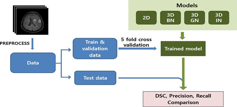
III. MATERIALS AND METHODS
This study utilized Python programming language version 3.7.12, TensorFlow framework version 2.7.0, as the backend for Keras version 2.7.0. Computational resources were provided by a Tesla T4 GPU (NVIDIA, Santa Clara, USA). Statistical analyses were performed using IBM SPSS Statistics for Windows version 27.
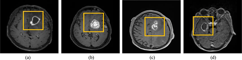
This study utilized MRI images from 600 patients with brain tumors at the Gachon University Gil Medical Center (IRB Number: GDIRB2021-192) (Fig. 1). The MRI technique used was T1 imaging, and the tumor label data were considered consistent when agreed upon by two radiologists. Among these, 400, 100, and 100 images were used as training, validation, and test data, respectively.
The patients consisted of 322 males and 278 females, with a mean age of 66.36±11.5 years and a median age of 66. The number of tumors in the patients varied from 1 to more than 26. Among them, 267 patients (44.5%) had 5 or fewer tumors, whereas 109 patients had 26 or more tumors. The median, mean, and standard deviation of the tumor counts were 7, 24.5, and 69.4, respectively (Table 1).
The tumor sizes in the patients varied from less than 100 mm3 to>3,000 mm3. The total number of tumors in the dataset was 26,400, with tumors smaller than 100 mm3 accounting for approximately 47.7% (12,600). The median, mean, and standard deviation of the tumor sizes were 123.3, 470.4, and 946.3, respectively (Table 2).
| Tumor size (mm3) | Number (n=26,400) | Ratio (%) | |
|---|---|---|---|
| Brain tumor size | =100 | 12,600 | 47.7 |
| 101−500 | 7,398 | 28.0 | |
| 501−1,000 | 2,400 | 9.1 | |
| 1,001−2,000 | 3,400 | 12.9 | |
| 2,001−3,000 | 800 | 3.0 | |
| Over 3,000 | 602 | 2.3 | |
The Pearson skewness coefficients for age, number of tumors per patient, and tumor size for all patients were 0.08, 0.75, and 1.1, respectively. Pearson skewness is an indicator of the asymmetry of data distribution, with positive values indicating right skewness and negative values indicating left skewness. The larger the absolute value, the greater the skewness. The Pearson skewness (Sk) was calculated using the following formula (1):
where Sk is Pearson skewness, X̅ is the sample mean, M is the median, and S is the standard deviation of the sample.
Nearest-neighbor interpolation was employed as a preprocessing technique to scale the images and normalize them to a size of 128×128×128 (Fig. 2).
The algorithm employed in this study is the Attention U-Net architecture. Attention U-Net is a model that enhances the performance by incorporating an attention gate algorithm into the conventional U-Net model [25].
Fig. 3 illustrates the architecture of the U-Net used in this study. U-Net utilizes convBlocks, in which the convolution-normalization-activation functions are sequentially arranged. For the convolution, similar to the conventional U-Net, 3×3×3 kernels with the same padding were applied to the 3D model, and 3×3 kernels were used for the 2D model.
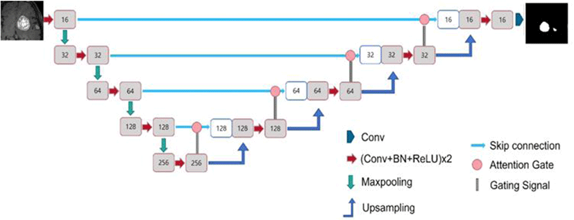
The conventional U-Net model employs batch normalization for the normalization layer. However, in this study, for 3D U-Net, in addition to the conventional batch normalization model, models using group and instance normalization were utilized (Fig. 4). The 3D models using batch, group, and instance normalization are referred to as the Batch normalization (BN), Group normalization (GN), and Instance Group normalization (IN) models, respectively. BN, GN, and IN represent batch, group, and instance normalization, respectively. The group size for group normalization was fixed at a default value of 32. The 2D model utilizes only batch normalization.
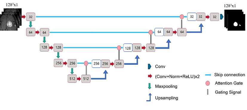
The original U-Net has 64 filters in its first convolution layer. However, based on the experimental results, it was determined that setting the number of filters in the first convolution layer to 16 for the 2D model and to 32 for the 3D model was more suitable. Therefore, the model was lightweight according to the findings of the preliminary experiments.
The dimensions, convolution filter numbers, and overall structure, excluding the normalization techniques, were the same for both the 2D and 3D U-Net models. The batch sizes for 2D and 3D U-Net were set to 128 and 1, respectively. Preliminary experiments confirmed that the 2D U-Net showed the best performance with a batch size of 128. For the 3D U-Net, it was impossible to increase the batch size due to memory limitations. The number of epochs was set to 200, as no further decrease in validation loss was observed beyond this point. The learning rate starts at 0.001 and is reduced by a factor of 0.3 whenever there is no significant decrease in the validation loss over five epochs. The initial learning rate was determined by experimenting with a wide range of values, including 0.05, 0.01, 0.005, 0.001 and 0.0005. The Adam optimizer was employed, and the loss function used was the Dice loss. The experiments were conducted using 5-fold cross-validation.
As a post-processing step, binarization was applied to the predicted masks obtained through model segmentation to remove noise.
In this study, image segmentation was conducted using both 2D and 3D artificial intelligence models, resulting in two types of predicted masks: 2D and 3D. Because the objective of this study is to compare the performance of the 2D and 3D U-Net models, for a fair evaluation, the predicted masks from the 2D model were merged into a 128×128×128 format to align with the dimensions of the 3D model.
The model performance evaluation utilized the average of 5-fold cross-validated DSC, precision, and recall as the evaluation metrics.
IV. RESULTS
3D GN and IN models exhibited higher DSC and recall values than those of the 2D model (p>0.05). The 3D IN model showed higher DSC, precision, and recall than the 3D GN model, but these differences were not statistically significant(p>0.05). The 3D BN model demonstrated a lower DSC and precision than the 2D model (p>0.05), whereas the recall was higher, although not statistically significant (p>0.05) (Table 3).
| Model | Mean±STD | ||
|---|---|---|---|
| DSC | Precision | Recall | |
| 3D BN | 0.73±0.054*▿ | 0.77±0.049*▿ | 0.75±0.37▿ |
| 3D GN | 0.77±0.016* | 0.82±0.008 | 0.78±0.019* |
| 3D IN | 0.78±0.014* | 0.82±0.016 | 0.78±0.013* |
| 2D | 0.74±0.009 | 0.82±0.009 | 0.73±0.011 |
According to the F-test results, the 3D BN model showed a statistically higher standard deviation in DSC, precision, and recall compared to the 2D BN model. In contrast, for the 3D GN and IN models, no statistically significant differences were observed compared to the 2D model in the F-test results (p>0.05).
The time required to segment the brain tumor image of one patient using the model was 96 ms, 110 ms, and 104 ms for the 3D model with batch, group, and instance normalization, respectively. By contrast, the 2D model took only 7 ms for the same segmentation task.
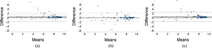
Fig. 5 shows a Bland–Altman plot comparing the DSC results of the 3D and 2D models. Although the average DSC of the 3D GN and IN models were higher than that of the 2D model, they did not consistently outperform the 2D model across all datasets. Similarly, although the average DSC of the 2D model was higher than that of the 3D BN model, there were instances in which the 3D BN model performed the segmentation better. Therefore, it was confirmed that a model with a higher average DSC might not necessarily perform better segmentation across all datasets.
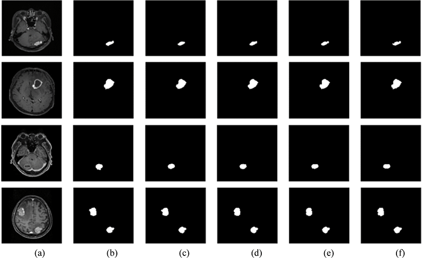
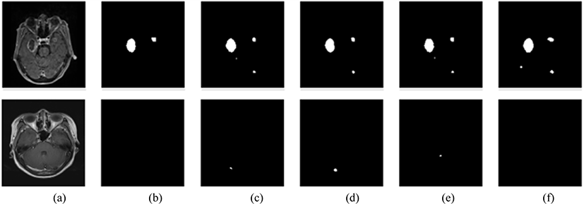
The model successfully segmented the images as shown in Fig 6. However, there were instances in which the segmentation accuracy was lower, as shown in Fig. 7.
V. DISCUSSION
In this study a performance comparison of brain tumor image segmentation was conducted using 2D and 3D U-Net models.
The 3D GN and IN models exhibited a higher DSC and recall than the 2D model, with no significant difference in precision. In contrast, the 3D BN model showed a lower DSC, precision, and recall than the 2D model. The 3D IN model demonstrated the highest DSC, precision, and recall among all the models, and the 3D GN model also showed a segmentation performance high enough to have no statistically significant difference compared with the IN model.
In terms of the F-test results for the standard deviation across folds, the 3D GN and IN models showed no significant differences compared to the 2D model. However, the BN model exhibited a considerably larger standard deviation than the 2D model.
Batch normalization smoothens the loss function during training, thereby aiding the model in effectively converging to a global minimum. However, in our experiment, the 3D model had a small batch size, rendering the batch normalization less effective. Therefore, the 3D BN model would have had difficulty converging to the global minimum. This is presumed to be a contributing factor to the observed low performance and high standard deviation of the 3D BN model.
However, models utilizing group normalization and instance normalization, which are not affected by batch size, appear to better leverage the potential of 3D structures.
Beyond the performance, notable distinctions were observed between the 3D GN and IN models and the 2D model. First, the 2D model struggled to effectively identify the upper and lower ends of the tumor compared with the 3D GN and IN models. This phenomenon is likely attributable to the tendency of brain tumors to have smaller cross-sectional areas towards the distal end. In slices at the distal end of the tumor, the tumor area can be very small, posing a challenge for the 2D model because it cannot leverage contextual information across slices. In contrast, 3D models that do not segment on a slice-by-slice basis exhibit a better tendency to segment the distal end of the tumor. The advantage of 3D models in utilizing context information across slices may contribute to improved performance as technology evolves or the dataset expands.
Second, the 3D model demonstrated a higher recall/precision ratio than the 2D model. It is crucial to detect all brain tumors during their diagnosis. However, a low recall implies a higher likelihood of overlooking existing tumors, potentially leading to the failure of early and accurate diagnosis.
In summary, the 3D GN and IN models outperformed the 2D model in terms of both overall performance and having a higher potential, particularly in achieving a relatively higher recall. However, its superiority over the 2D model was not consistent across all aspects.
The 2D model exhibited advantages in terms of training time, requiring more than twice the time per step during training, and the application time was more than 13 times shorter than that of the 3D models.
Additionally, as evident in the Bland Altman plots, it was not always the case that the 3D GN and IN models consistently outperformed the 2D model in segmentation; in some instances, the segmentation by the 2D model was more accurate. Because 3D models can utilize information between slices, they are likely to have higher accuracy in regions where inter-slice information is important. However, due to the greater complexity of the model, they may be more prone to overfitting, which could explain the lower performance in specific cases. Complex models require more data for adequate generalization, indicating that more data would be necessary [26]. Additionally at this stage, it would be beneficial to leverage the advantages of both 2D and 3D structures, possibly through hybrid approaches that incorporate both structures.
In this experiment, the DSC, precision, and recall of the AI segmentation results were not high compared to those in other studies. This could be attributed to the fact that the dataset used in this experiment contained numerous images of small and abundant brain tumors compared to the datasets used in other studies.
Additionally, the group size for group normalization was fixed at a default value of 32. Therefore, future research should involve experiments with a larger dataset, experiments using brain tumor images with, on average, larger sizes, and experiments comparing different group sizes for group normalization.
As advancements in technology may enable the use of larger batch sizes in 3D U-Net models in the future, further experiments will be necessary to determine which normalization layer will be the most effective under those conditions.
VI. CONCLUSION
A comparison of 2D U-Net and 3D U-Net for brain tumor image segmentation in this study revealed that the best performance was achieved by 3D U-Net utilizing group or instance normalization.
Therefore, when using 3D U-Net, if a large batch size cannot be used, it is effective to use instance normalization (IN) or group normalization (GN) instead of batch normalization.
Subsequent studies should explore more extensive datasets, larger tumor sizes, and varying group sizes for group normalization.